Pump performance curves look intimidating at first glance, yet they are among the most practical tools for sizing, troubleshooting, and operating pumps; understanding them is easier when pump curves are explained clearly. With a bit of structure and a few worked examples, the shapes, intersections, and numbers on these charts start to tell a clear story about what a pump can and cannot do.

The notes below focus on centrifugal pumps, since they dominate water and process duties. The same logic helps a junior technician set a duty point in the field and helps an engineering student make solid design choices on paper.

What a pump curve shows

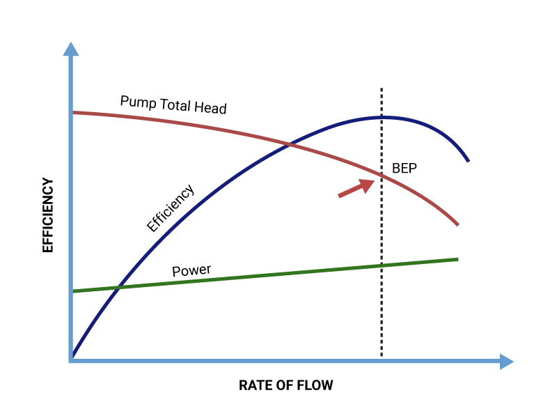
A standard centrifugal pump curve bundles several plots on the same chart:

• Head versus flow rate, also known as H-Q
• Efficiency versus flow
• Power input versus flow, typically labeled brake horsepower or kW
• Required net positive suction head, NPSHr, versus flow
• A mark for best efficiency point, BEP

A single catalog page usually shows multiple impeller diameters and sometimes multiple speeds. Each H-Q curve slopes downward. Near zero flow, the pump produces its highest head, often called shutoff head. At runout, where the curve approaches maximum flow, head is lower and efficiency usually drops.

The other overlays place a second layer of meaning on top of H-Q. Efficiency peaks near BEP. Power input often rises with flow. NPSHr usually increases with flow, and it must be compared with the system’s available NPSH, NPSHa, to avoid cavitation.

Head versus flow

Head is energy per unit weight. It indicates how high a pump can raise a fluid column and is independent of density, which makes it a convenient measure. In US practice, head is plotted in feet; in SI, meters.

Several points to recognize on H-Q:

• Shutoff head at zero flow
• The falling head trend as flow increases
• Runout where stable operation ceases
• A stable region bounded by minimum continuous stable flow on the low side and an upper limit on the high side

Why head drops with flow is tied to internal losses and velocity changes inside the impeller and volute. The exact curve shape depends on blade geometry, specific speed, and diffusor design.

A simple energy balance still helps. For a control volume around the pump:H_pump = ΔP/(ρ g) + ΔV^2/(2 g) + ΔzPump curves provide H_pump directly, so designers can focus on how the system requires head at any flow.

Efficiency curve

Pump efficiency compares hydraulic output to mechanical input, highlighting the importance of hydraulics in evaluating performance. It captures blade incidence, disc friction, leakage across wear rings, and many other loss sources in a single number. The efficiency curve rises, peaks at BEP, then falls. Operating too far off BEP increases vibration, noise, bearing loads, and seal stress. Manufacturers often highlight an allowable operating window around BEP where reliability and energy use remain reasonable.

In practice, sizing to put the duty point near BEP pays back in power savings and longer component life.

Power curve and motor sizing

The power plot shows input power to the pump shaft. Catalogs express this as brake horsepower or kW at the pump shaft, not the motor shaft. The familiar water horsepower relation in US units is:HP_hydraulic = Q gpm × H ft × SG / 3960BHP at the shaft is higher, since BHP = HP_hydraulic / η_pump.

Two reminders:

• Motor nameplate power must exceed expected BHP with margin for service factor, temperature, and voltage variation.
• Viscous or slurry service raises required power beyond water tests, so derating factors or corrected curves should be applied.

NPSHr and cavitation

NPSHr is derived from shop testing with cold water and a controlled drop in suction head until performance degrades by a defined amount. It is not the suction head the pump prefers to have; it is the minimum the pump requires to avoid a measurable drop-off.

The system provides NPSHa. In US units, a common form is:NPSHa = P_abs at liquid surface in feet of water + z_suction − h_f,suction − H_vapor

• P_abs in an open tank equals atmospheric head, about 33.9 ft at sea level
• z_suction is liquid level above the pump datum, positive if above
• h_f,suction is friction loss from surface to impeller eye
• H_vapor is the vapor pressure head of the fluid at operating temperature

Safe practice keeps NPSHa comfortably above NPSHr, often by a margin factor set by company standard or the Hydraulic Institute, especially where suction transients or higher temperatures are expected.

Best efficiency point and operating range

BEP is the flow at which hydraulic losses balance most favorably. Besides power savings, operation close to BEP reduces radial thrust on the impeller. That thrust peaks when the pump is pushed far left or right on the H-Q curve, which shortens bearing and seal life. Many OEMs provide a preferred operating range around BEP, for example 70 to 120 percent of BEP flow for clear liquids, sometimes narrower for high specific speed machines or low specific speed units.

Selecting a pump that places the duty point near BEP is not just about efficiency. It is a reliability decision.

A quick reference table

System curve and finding the duty point

A system requires head to overcome two contributors and ensure optimal application:

• Static head, the elevation change between source and destination, plus any static pressure difference between the two
• Friction head, which grows approximately with the square of flow in turbulent regimes, including pipe friction and minor losses through valves and fittings

That relationship is often written as:H_system(Q) = H_static + K Q^2K captures pipe roughness, length, diameter, and minor loss coefficients. For closed loops with the same free surface or expansion tank pressure at suction and discharge, static head cancels and H_system is mostly friction.

The operating or duty point is the intersection of H_pump(Q) and H_system(Q). On a chart, technicians draw the system curve and see where it crosses the pump curve. In a spreadsheet, they solve H_pump(Q) = H_system(Q) for Q.

A short field method to sketch a system curve:

1. Estimate H_static from drawings or level readings
2. Compute friction at a reference flow using Darcy–Weisbach or Hazen–Williams
3. Back-calculate K from H_f,ref = K Q_ref^2
4. Express H_system(Q) = H_static + K Q^2
5. Overlay on the pump curve to find the intersection

Throttle valves change the system curve by adding loss, which alters flow rate and shifts the duty point left along the pump curve. Variable speed changes the pump curve itself, which often keeps operation near BEP while matching demand.

How speed and impeller diameter shift the curve

Affinity laws give quick estimates when speed or impeller diameter changes are small.

At fixed diameter and varying speed n:

• Q2 = Q1 × n2/n1
• H2 = H1 × (n2/n1)^2
• P2 = P1 × (n2/n1)^3

At fixed speed and small diameter change D:

• Q2 = Q1 × D2/D1
• H2 = H1 × (D2/D1)^2
• P2 = P1 × (D2/D1)^3

These relations help set VFD speeds and anticipate motor load, and they allow a designer to test whether a smaller trimmed impeller will meet the same duty.

Worked example 1: water circulation in a building loop

Goal: Estimate the duty point, NPSH check, and motor size for a chilled water loop.

Assumptions

• Fluid: water at 100 F, SG ≈ 1.0
• Closed loop, expansion tank keeps loop pressure at 12 psig at the pump suction header
• Target flow near 200 gpm
• Pipe: 4 inch steel, 400 ft equivalent length around the loop, including fittings
• Suction piping to pump eye: 8 ft of 6 inch pipe with two large radius elbows

Step 1. System curve

• Static head for a closed loop cancels for the circulating pump, so take H_static ≈ 0 ft
• Use Hazen–Williams with C = 120 to estimate loop friction, considering hydraulics principles. At 200 gpm in 4 inch pipe, the loss is around 6.2 ft per 100 ft, so about 24.8 ft for 400 ft. At double flow, friction rises roughly by a square factor
• Build a quadratic model H_system(Q) = K Q^2 with K set by 24.8 ft = K × 200^2 → K = 24.8/40000 = 0.00062 ft/(gpm^2)

Result:H_system(Q) = 0.00062 Q^2

Step 2. Candidate pump curveAssume a catalog pump at 1750 rpm with an impeller that can be approximated near the expected duty by:H_pump(Q) = 110 − 0.0012 Q^2

Step 3. Duty point from intersectionSet 110 − 0.0012 Q^2 = 0.00062 Q^2 to determine the total dynamic head required for the system.110 = 0.00182 Q^2 → Q ≈ 246 gpmHead at duty: H ≈ 0.00062 × 246^2 ≈ 37.5 ft

Step 4. Efficiency and powerAssume the pump’s efficiency curve peaks at 78 percent near 250 gpm and is 77 to 79 percent in that region. Take η = 78 percent.

BHP = Q H SG / (3960 η) = 246 × 37.5 × 1.0 / (3960 × 0.78)BHP ≈ 9209 / 3089 ≈ 3.0 hp

A 5 hp motor provides adequate margin.

Step 5. NPSH check

• NPSHr at 246 gpm from the catalog curve: assume 8 ft
• NPSHa from loop pressure and suction losses:
• Loop pressure at suction header: 12 psig → 12 × 2.31 = 27.7 ft
• Static height of liquid above pump eye: 3 ft
• Suction line friction and fittings to pump: estimate 4 ft
• Vapor head at 100 F: about 1.9 psia → 1.9 × 2.31 = 4.4 ftNPSHa ≈ 27.7 + 3 − 4 − 4.4 = 22.3 ft

With NPSHa well above 8 ft, cavitation margin is comfortable.

Observations

• The operating point sits near BEP, so reliability and energy performance should be favorable
• A VFD could trim speed to match minor seasonal changes while keeping operation near the high efficiency region

Worked example 2: slurry transfer from a pit to a thickener

Goal: Size a pump for a mineral slurry with higher friction and higher power draw than water.

Assumptions

• Fluid: sand slurry with SG = 1.20, medium solids loading with modest settling tendency
• Required flow near 500 gpm
• Suction source: open pit with flooded suction, pump centerline 6 ft below liquid level
• Discharge destination: thickener feed box 40 ft higher than pump centerline
• Line: 6 inch rubber lined steel, 1000 ft equivalent length
• Use a simplified water friction baseline with a correction factor for slurry

Step 1. System curve

• Static head H_static = 40 ft
• Water friction at 500 gpm in 6 inch: about 30 ft for 1000 ft equivalent (illustrative)
• Apply a slurry friction factor of 1.3 for this mixture and velocity range: 30 × 1.3 ≈ 39 ftSet K by 39 = K × 500^2 → K = 39/250000 ≈ 0.000156 ft/(gpm^2)

H_system(Q) = 40 + 0.000156 Q^2

Step 2. Candidate pump curveAssume a pump at 1780 rpm with:H_pump(Q) = 120 − 0.00012 Q^2

Step 3. Duty pointSolve 120 − 0.00012 Q^2 = 40 + 0.000156 Q^280 = 0.000276 Q^2 → Q ≈ 538 gpmHead at duty: H ≈ 40 + 0.000156 × 538^2 ≈ 85 ft

Step 4. Efficiency and powerTake water efficiency at this flow as 72 percent. Apply a slurry correction factor to efficiency of 0.9. Effective η ≈ 0.72 × 0.9 = 0.648.

BHP = Q H SG / (3960 η) = 538 × 85 × 1.20 / (3960 × 0.648)Numerator ≈ 538 × 85 × 1.2 ≈ 54,900Denominator ≈ 3960 × 0.648 ≈ 2566BHP ≈ 21.4 hp

A 30 hp motor is prudent to provide margin for solids variability, wear, and speed adjustments.

Step 5. NPSH check

• NPSHr at 538 gpm from water test: assume 12 ft
• Apply a modest slurry factor, say 1.1 → effective requirement ≈ 13.2 ft
• NPSHa with open pit suction:
• Atmospheric head at sea level: 33.9 ft
• Static submergence above pump eye: 6 ft
• Suction line friction: 5 ft
• Vapor head at 70 F: about 2.3 ftNPSHa ≈ 33.9 + 6 − 5 − 2.3 = 32.6 ft

With NPSHa well above the adjusted requirement, the suction condition is acceptable.

Observations

• The operating point is right of the pump’s BEP for water, and efficiency is reduced by the slurry. Oversizing the motor by a healthy margin avoids nuisance trips
• Wear will enlarge clearances and shift the pump curve downward over time. Monitoring flow and head can signal when re-trim or overhaul is due

Reading and using curves step by step

Students and technicians often benefit from a checklist:

• Define the fluid: SG, viscosity, temperature, solids type and loading; consider the total dynamic head needed for the system.
• Draw the hydraulic path to separate static head from friction head
• Estimate friction at a reference flow and construct H_system(Q) = H_static + K Q^2
• Overlay H_system with candidate H_pump curves for available models, diameters, and speeds
• Pick a duty point near BEP where NPSHa exceeds NPSHr with margin
• Read efficiency and power at the duty point and select a motor with suitable service factor
• Test sensitivity with speed changes using the affinity laws
• Consider control strategy. Throttling adds loss. VFDs move the pump curve while keeping operation efficient

Common pitfalls

• Chasing head by throttling until noise appears, which often means cavitation or operation far left of BEP
• Ignoring suction piping losses when calculating NPSHa
• Forgetting that catalog NPSHr is from cold water tests and that warm fluids or slurries need extra margin
• Assuming closed loops have zero head always. They have zero static head for the circulating pump but often high friction head
• Over-reliance on nameplate flow numbers instead of reading the intersection on the actual curve

FAQs

Q1: Why do some pumps have very flat H-Q curves while others drop steeply?

A1: Shape is tied to specific speed and hydraulic design. Low specific speed pumps with radial flow impellers tend to show steeper head drop. Higher specific speed designs closer to mixed or axial flow appear flatter. Flat curves can be helpful for level control, while steep curves can be more forgiving for parallel operation.

Q2: How close to BEP should a duty point be in practice?

A2: Many facilities aim for 80 to 110 percent of BEP for general service water pumps. Some API and ANSI process pumps operate comfortably in a similar window, though exact limits depend on bearing design and hydraulic layout. Requirements for multistage or very low specific speed machines can be tighter. OEM recommendations take precedence.

Q3: What is the difference between NPSHr and minimum submergence on a vertical pump?

A3: NPSHr is a pump characteristic measured on a test stand that reflects when performance degrades due to cavitation. Minimum submergence is a system requirement that ensures a vertical pump’s inlet remains deep enough below the liquid surface to prevent vortices and air entrainment. Both must be satisfied. Submergence helps control air ingestion; NPSH margin protects against cavitation inside the pump.

Short reminders for field work

• Confirm liquid level and suction pressure before declaring a pump undersized
• If a VFD is available, test a few speeds and record flow, head, amps, and noise to locate a stable operating window
• Keep a record of bearing temperature and seal leakage when operating away from BEP

Pump curves reward careful reading. Engineers and technicians who practice the steps above tend to make fast, accurate calls in the field and during design. To go deeper into examples, worksheets, and interactive curve building, they can explore more lessons at Pump Systems Academy.