How to Use Pump Curves, System Curves, and Affinity Laws to Optimize Performance

Every pump delivers what its hydraulics and the connected piping allow, not what the nameplate promises. Real savings and reliability come from placing the operating point where the pump and the system agree, then shaping that point with speed or impeller diameter. The tools are simple: read the pump curve, plot the system curve, and apply the Affinity Laws with discipline.

Pump curves: the map of delivered performance

A factory pump curve is a set of test data organized so that flow, head, efficiency, power, and NPSHr can be read for any operating point within the tested range. It is not a theoretical ideal. It is a fingerprint of a specific hydraulic design running at a stated speed, fluid, and impeller diameter.

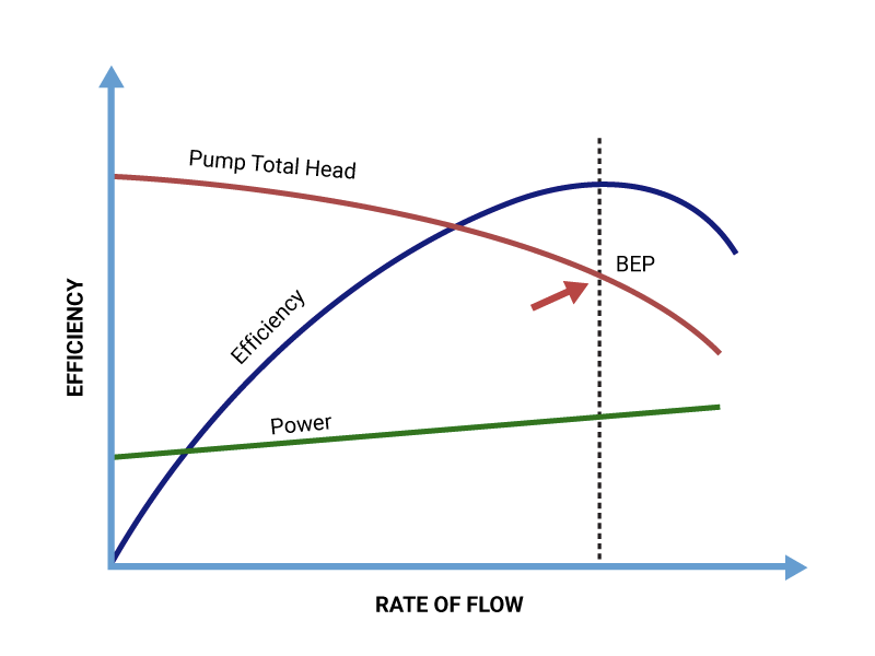
Most curves present head on the vertical axis and flow on the horizontal axis. Efficiency lines drape across the chart, forming bands where the pump uses input power most effectively. The peak of those bands identifies the Best Efficiency Point. At BEP, internal hydraulic forces are balanced, radial thrust is lower, and vibration tends to be minimal.

Operating near that sweet spot has outsized value. Bearings and seals last longer, energy use drops, and noise declines. Move far left or right and the pump may still meet a flow target, but with penalty in shaft deflection, recirculation, and wasted power.

A modern performance sheet also includes several other curves and overlays that deserve careful attention.

• Head vs. flow: the primary curve that shows how much head the pump can generate at each flow point.
• Efficiency bands: iso-efficiency lines that show where the pump converts shaft power into hydraulic power most effectively.
• Power draw: expected brake horsepower or kilowatts at each operating condition.
• NPSHr: the minimum suction head the pump requires to avoid cavitation during testing conditions.

Two identical pumps from the same series can have different curves after trimming the impeller. A curve always ties to speed, diameter, and fluid properties that match the test basis.

System curves: what the piping demands

Where the pump curve expresses supply, the system curve expresses demand. It captures how much head the piping and process require at each flow rate. Static elevation creates a vertical shift, while friction losses grow with the square of flow, bowing the curve upward.

Static head is set by geometry. A tank-to-tank transfer that lifts liquid by 20 feet imposes that 20 feet at any flow rate. Friction depends on pipe size, roughness, length, and the catalog of fittings and valves. Engineers choose Darcy–Weisbach, Hazen–Williams, or manufacturer loss coefficients. Either approach, if applied consistently, will produce a usable relation between flow and head.

The system curve is not fixed forever. Valves change position, pipelines foul, and slurries thicken. Temperature changes viscosity. A curve built from design drawings can drift in the field over months.

After building the baseline relation, many operators keep a small toolkit of field checks, for example differential pressure readings across a known restriction or ultrasonic flow measurements during testing. Those points let them confirm whether friction has shifted.

A few practical shifts help translate chart motion to plant actions:

• Opening a control valve pushes the system curve downward.
• Closing a valve pushes it upward.
• Adding pipe, fouling, or tighter strainers moves the curve upward.
• Removing restrictions or cleaning exchangers moves it downward.

Even simple sketches with three or four points can reveal enough to choose a control strategy.

Where pump and system meet: the operating point

Place the system head curve on top of the pump curve referenced to the same speed and impeller diameter. Their intersection defines the actual operating point. That single point sets delivered flow and the total dynamic head the pump must produce.

If the intersection sits left of BEP, expect higher radial loads, increased recirculation on the suction side, and noise. If it sits far right, NPSH margin often shrinks while power climbs. Both sides eat into reliability.

Plant engineers often manage an operating envelope, not a single point. Seasonal changes, variable tank levels, or batch operations move the system curve through a range. Designing for a broad region around BEP pays dividends. That may mean selecting a pump with a flatter curve or a different specific speed to hold efficiency across the expected flow range.

A one-sentence rule captures this section: the system chooses the point, the pump only offers the curve.

The Affinity Laws in practice

The Affinity Laws predict how performance scales when speed or impeller diameter changes, assuming the same pump, the same fluid, and a similar efficiency region. They are approximations that hold well within a reasonable window.

The proportionality is compact and easy to apply. Flow scales linearly with speed and diameter. Head scales with the square. Power scales with the cube.

The table below summarizes the relationships and gives quick estimates for common adjustments.

Small changes compound quickly for power. A modest drop in speed can yield a large cut in energy consumption while still meeting process needs.

When applying the laws, keep the operating region in mind. Large moves can shift the pump into a less efficient part of the curve, change NPSHr, and alter internal recirculation patterns.

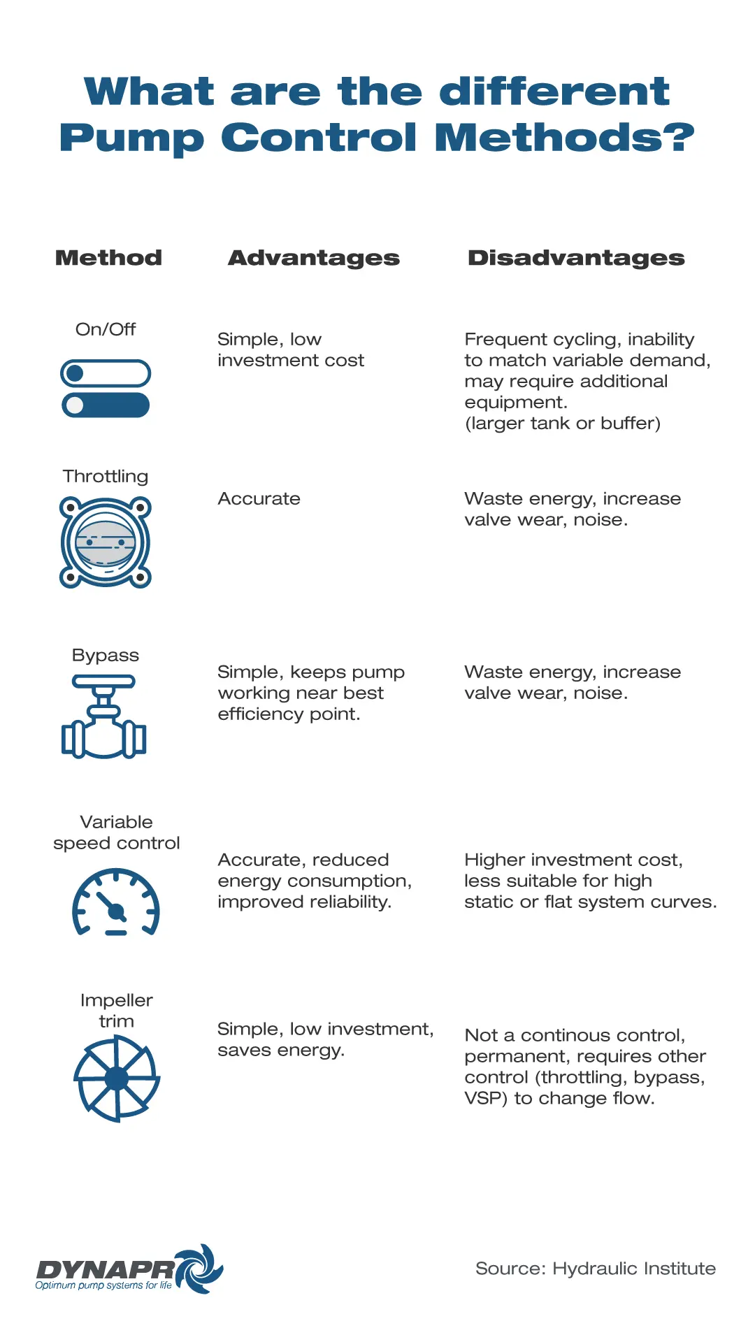
Choosing control strategies: speed, diameter, or throttle

Variable speed drives transform how pumps are controlled. Speed reduction lowers flow and head in a predictable way, often keeping the operating point near BEP while reducing power. By contrast, throttling a discharge valve holds speed constant and forces the system curve upward. The pump remains at a higher power draw even though delivered flow drops.

Impeller trimming offers a permanent change, attractive when the process has a stable requirement lower than the original design. Trimming shifts the entire pump curve downward. Efficiency usually stays acceptable if the trim is not extreme, and the operating point can sit closer to BEP than with heavy throttling.

A short example makes the contrast clear. Consider a pump at 1800 rpm delivering 1000 gpm at 140 ft with 160 hp. If a process only needs 800 gpm, two choices exist:

• Throttle: move up the system curve until flow reads 800 gpm. Head rises, power often stays near 150 to 160 hp, and BEP deviation grows.
• Speed control: reduce speed using Affinity Laws, target Q at 800 gpm with N scaled to 0.8 of original. Head target becomes 0.64 of original, power falls near 0.512 of original, close to 82 hp. Field numbers will differ, but the direction and magnitude are consistent.

Permanent needs suit trimming. Variable needs suit speed control.

Building a system curve that matches reality

Textbook friction calculations start the process, yet good practice adds field fingerprints. Operators often log:

• Static level differences during startup and full drawdown.
• Differential pressure across known fittings or strainers.
• Flow meter readings at several valve positions.

With those points in hand, a revised system curve can be fitted. If recorded head at a given flow is higher than the original estimate, fouling or an undersized line may be present. If lower, a mistakenly oversized pump or a bypass path may exist.

One subtlety deserves mention. Many systems have two regimes, one dominated by static head and another dominated by friction. Tank transfer to a high vessel has a large vertical lift. Once elevation is overcome, friction sets the shape, and relative energy savings from speed control are greater.

NPSH, cavitation, and suction limits

NPSH margin is the counterpart of speed and diameter changes on the suction side. NPSHr curves are measured on cold water in a test lab and reflect the point where a 3 percent head drop appears. That point is not a comfort zone for real fluids.

High viscosity or vapor pressure reduces NPSHa. Hot hydrocarbon services or near boiling water at elevation warrant a proper margin policy, often NPSHa at least 1 meter above NPSHr for water and more for hot or flashing liquids. Some plants adopt a percentage margin instead.

Speed changes affect NPSHr, typically moving it upward with increased flow. Any change that chases more flow to the right will tighten NPSH margin. Impeller inducer designs and low specific speed impellers can temper the trend, yet they do not remove it.

Listening for noise, tracking vibration near the suction side, and checking for pitted impellers or mechanical seal distress remain the field clues when instrumentation is limited.

Putting curves and laws to work: a repeatable workflow

Optimizing a pump rarely starts with a blank spreadsheet. It starts with a baseline.

First, collect the pump curve for the exact model, impeller diameter, and nominal speed. Note the efficiency bands and BEP location. Confirm the units and reference fluid.

Second, assemble the system description. Elevation difference between source and destination, pipe diameters and lengths, dominant fittings, control valve Cv and position, strainers or exchangers that add head. Build a clean system curve from those inputs.

Third, find the intersection. Mark the operating point. Read efficiency, power, and NPSHr at that point. Compare with the duty requirement.

Fourth, evaluate control options. If flow is higher than needed, try an Affinity Laws speed reduction and replot. If the process is steady and long term, assess an impeller trim that relocates the pump curve so the intersection sits near BEP. Keep NPSH margin in view for any rightward shift.

Fifth, validate with field data. Small test steps with a temporary flow meter or differential pressure gauge can confirm the shape and position of the system curve. Update calculations based on measured points.

Finally, document the new normal. Record the expected speed at key flows, the available margin, and the alarm thresholds for vibration, temperature rise, and suction stability. Those notes prevent the next shift from drifting back to throttle control when a quick fix tempts them.

Accounting for fluids and temperature

Water-based curves set a baseline. Real services move far away from that baseline.

Viscous fluids change the pump’s internal losses and efficiency. The effect is not just increased friction in the pipes. Correction methods, like the Hydraulic Institute viscosity correction charts, adjust head, flow, power, and efficiency estimates to match higher viscosity. Ignoring viscosity often leads to undersized motors or short-lived seals.

Slurry services add solids and density. Increased density raises power for a given head and flow, and abrasive particles accelerate wear, changing the curve over time. A system that looks balanced on day one may drift within weeks if the hydraulic passages erode.

Temperature shapes vapor pressure and NPSH. Elevated temperature raises vapor pressure, which shrinks NPSHa. Elevation above sea level reduces absolute pressure on the suction side as well. Both factors erode cavitation margin and deserve specific calculation.

In short, never carry over a cold-water curve to hot, viscous, or two-phase services without correction.

Diagnosing problems with curves

Curves are not only design aids. They serve as diagnostic tools when performance degrades.

If flow drops while measured head stays similar, the system curve likely moved upward, often due to fouling or a partially closed valve. If head drops with similar flow, impeller wear or recirculation damage may be present. If power rises sharply at the same flow, liquid density or viscosity might have changed.

A small set of trend plots makes pattern matching easier: suction pressure, discharge pressure, motor amps or kilowatts, and control valve position. Overlaying those with expected intersection points can quickly show whether the pump curve moved, the system curve moved, or both.

Common mistakes that drain money

Many recurring issues trace back to a handful of avoidable errors. After one short paragraph, a compact list helps with review.

• Selecting by flow alone
• Ignoring NPSHr and cavitation margin
• Using nameplate performance without field confirmation
• Relying on throttle-based control for continuous turndown
• Skipping viscosity or slurry corrections
• Forgetting that system friction changes with fouling

Each item looks small in isolation. Together they shorten equipment life and inflate energy bills.

Short case example: quantifying savings from speed control

A chilled water pump rated 2000 gpm at 100 ft head runs at 1800 rpm with 85 percent pump efficiency at BEP. Building load during weekends drops to 1200 gpm, yet the plant historically holds speed constant and throttles a valve to maintain flow.

Applying the Affinity Laws, the target speed to deliver 1200 gpm near the same portion of the curve is 0.6 of original, about 1080 rpm. Head scales to 36 ft and, if the system allows, that becomes the operating point. Power scales with the cube, so the pump’s hydraulic power falls to roughly 0.216 of the original. Even with motor and drive losses, energy use plunges.

The VSD also keeps the operating point closer to BEP for much of the week. Vibration history improves, and seal mean time between failures extends. The capital cost of the drive soon pays back through reduced electrical consumption and maintenance labor.

FAQs

Why do pump curves and system curves matter?

They determine the actual operating point, which sets delivered flow, head, efficiency, and reliability. A poorly placed intersection raises energy use and mechanical stress.

Can the Affinity Laws be used for real-time adjustments?

Yes. With a VSD, speed changes can be predicted and tested safely in small steps. Operators often validate a few points, then rely on the scaling for routine setpoints.

Are pump curves identical across models?

No. Each pump family has its own hydraulics, specific speed, and efficiency bands. Even within one family, impeller trims shift the curve.

What are the risks when operating far from BEP?

Expect higher vibration, more radial thrust, increased seal and bearing loads, and lower efficiency. Cavitation risk can also rise if the shift moves the duty point rightward into higher flow with limited NPSH margin.

How does training change day-to-day results?

Teams that read curves, fit system curves from field data, and apply the Affinity Laws make better control decisions. That translates into lower energy bills, fewer emergency repairs, and more predictable production.