Pump Affinity Laws: Formulas & Engineering Guide

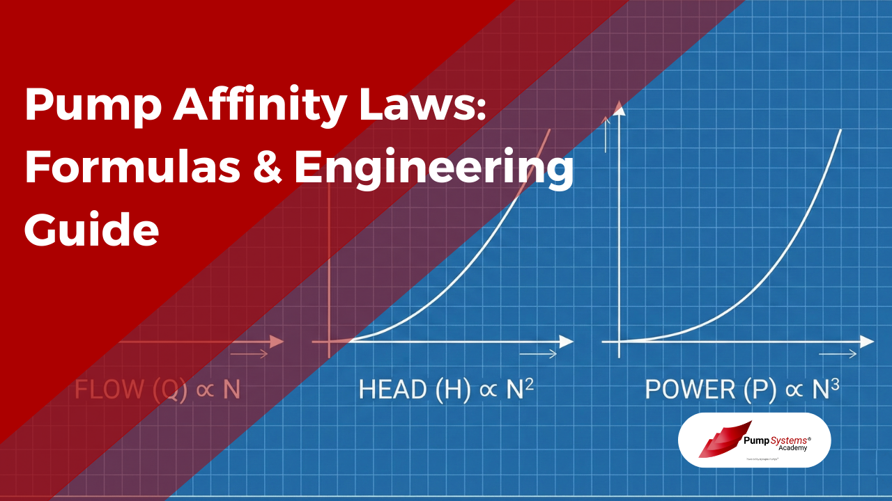
A set of quick, reliable scaling rules can save hours in pump selection meetings and prevent expensive trial and error in the field. The pump affinity laws do exactly that for centrifugal, rotodynamic pumps: they estimate how flow, head, and power change when speed or impeller diameter changes. Students use them to interpret pump curves, maintenance planners use them to evaluate VFD projects, and process engineers use them to sanity-check operating points against the system curve.

Used well, they explain why a small RPM reduction can cut brake horsepower (BHP) dramatically. Used poorly, they can hide the static head trap and lead to a pump that simply cannot lift the liquid.

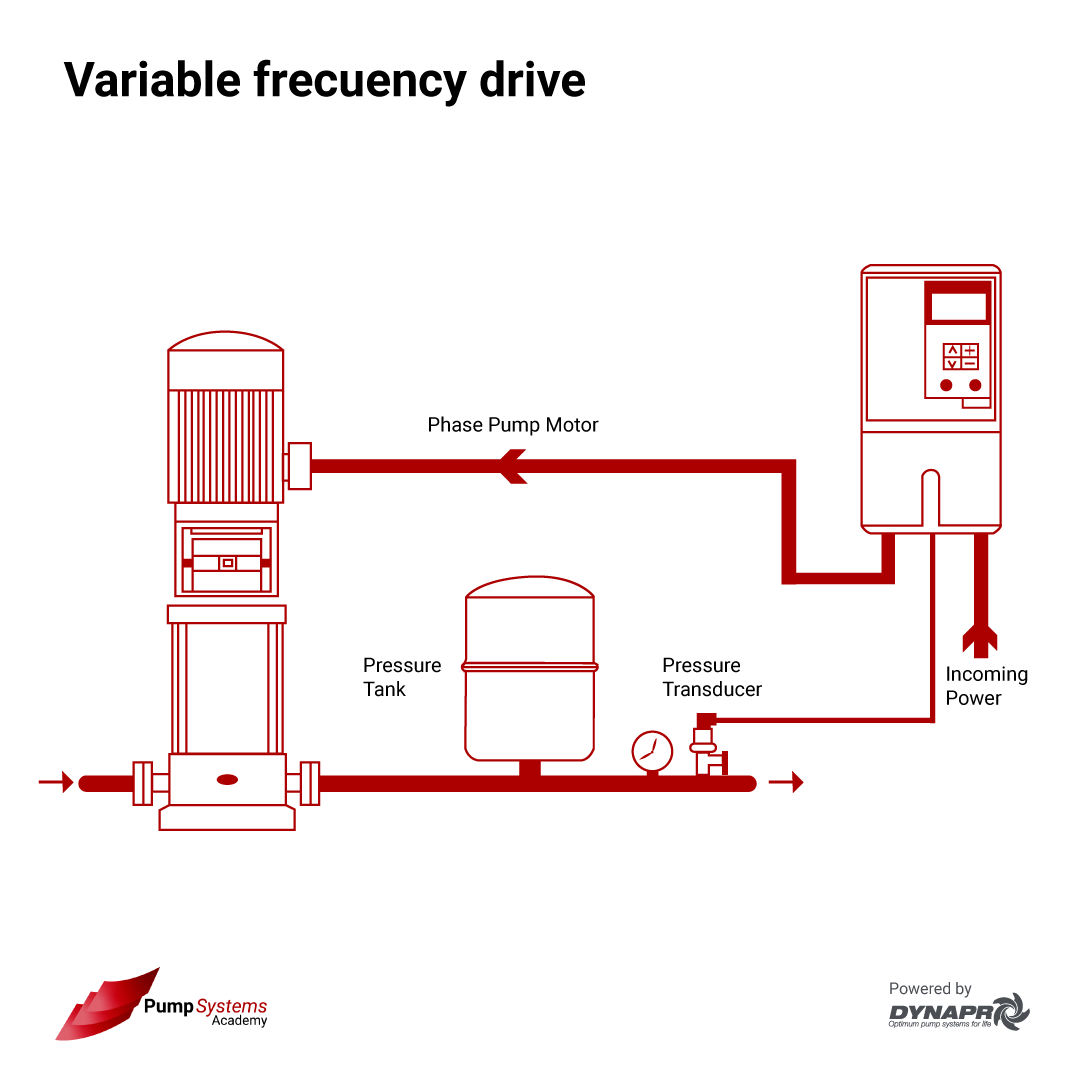
The reason these laws matter is practical: most plants do not need maximum flow all the time. If the process demand varies and the pump speed is adjustable via a variable frequency drive (VFD), the operating point can be shifted without throttling away energy as friction loss across a control valve.

A second reason is corrective: if a pump is consistently oversized, impeller trimming can move the pump curve down to match the actual duty, lowering dynamic head and power draw while keeping the piping unchanged.

What Are the Pump Affinity Laws?

The pump affinity laws are proportional relationships that predict how a centrifugal pump’s performance changes when either rotational speed (RPM) or impeller diameter changes, assuming the pump remains geometrically similar and operates in a comparable flow regime.

They are built on similarity principles used across rotodynamic machines. In plain terms, tip speed sets the velocity imparted to the fluid; velocity drives head; and hydraulic power is tied to flow times head divided by hydraulic efficiency. When the pump is scaled by speed or diameter, the resulting changes follow predictable exponents.

After a pump curve exists at one condition, these laws let an engineer estimate a new curve and then intersect it with the system curve to find the new operating point.

Relationship Between Speed (RPM), Flow, and Head

For speed changes at constant impeller diameter, the classic “three rules” are:

• Flow (Q) changes directly with speed (N).
• Head (H) changes with the square of speed.
• Power (P) changes with the cube of speed.

Those rules describe the pump side. Real systems add the system curve, typically modeled as:

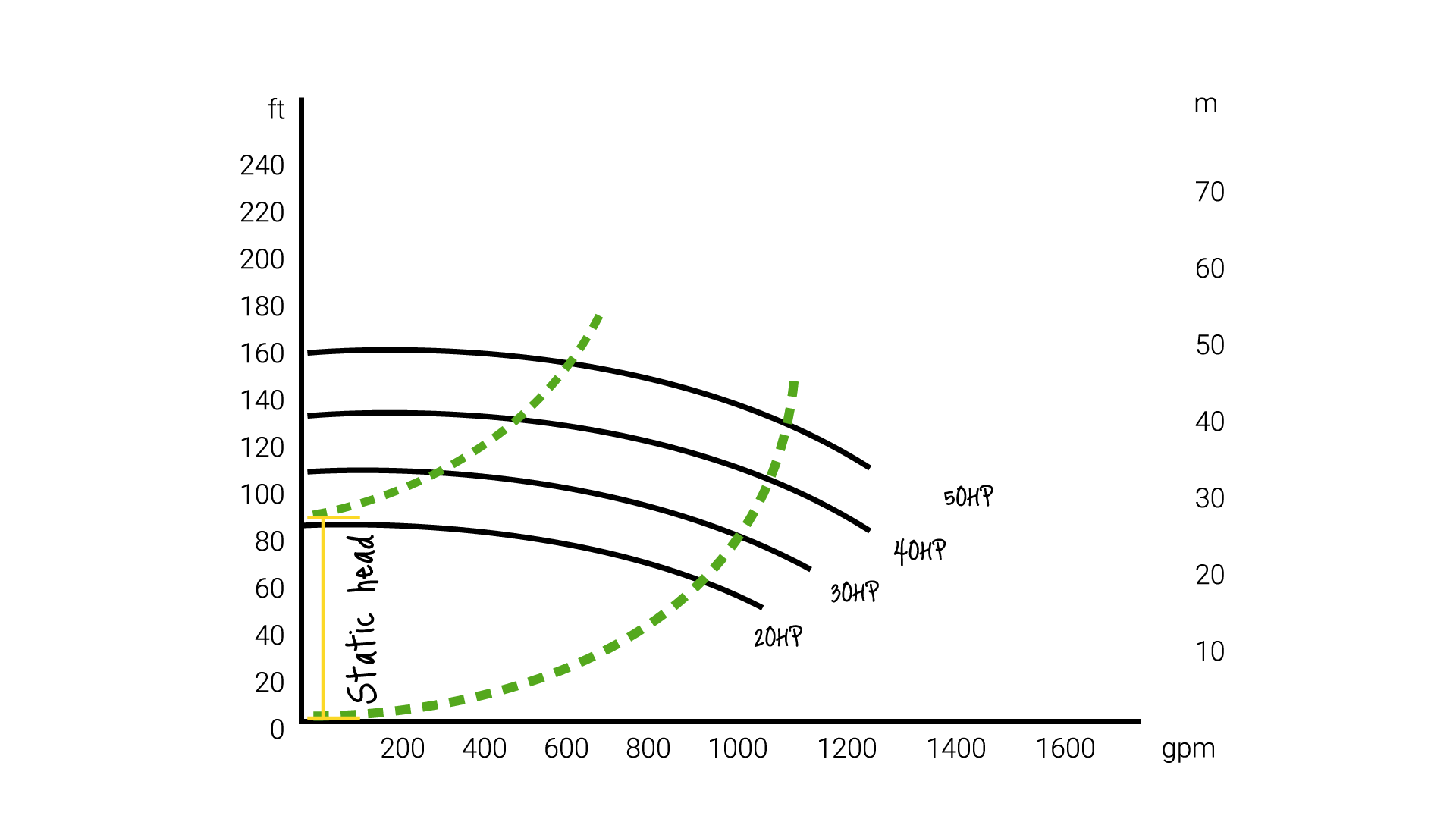
System head = static head + friction headFriction head is often proportional to Q^2 in turbulent flow, which is common in process piping.

A helpful mental model is that speed changes “scale” the pump curve, while the system curve usually stays fixed in shape. The actual operating point shifts to the new intersection, which can differ from the simple Q ∝ N estimate if static head is significant.

The "Cube Law": How Speed Affects Power Consumption

The cube law is the headline result for energy savings: at constant impeller diameter and roughly similar hydraulic efficiency, shaft power varies with the cube of speed.

That means modest speed reductions can produce large reductions in BHP. It also means speed increases can overload motors quickly if the margin is small.

After a paragraph of math, it becomes intuitive. Hydraulic power is proportional to Q * H. If Q ∝ N and H ∝ N^2, then Q * H ∝ N^3. Real motor input power adds drive and motor efficiencies, but the cubic trend still explains why VFD control is so effective in variable-flow services.

A small set of implications tends to show up repeatedly in plant studies:

• Energy savings: small RPM reductions can cut kW sharply.
• Control strategy: VFD speed control often beats throttling when friction losses dominate.
• Risk check: raising speed even 5% to 10% can push power and NPSH limits.

Affinity Laws for Impeller Diameter Changes

Impeller diameter changes, including impeller trimming, follow the same exponent pattern as speed changes because they also change tip speed. For a fixed RPM:

• Q scales with diameter (D).
• H scales with D^2.
• P scales with D^3.

In maintenance and reliability work, trimming is a common corrective action when the pump is oversized and a permanent reduction in duty is acceptable. It is not simply “free efficiency,” though. Large trims can shift the best efficiency point (BEP), alter internal recirculation patterns, and change vibration behavior.

A conservative workflow is to estimate the new performance with affinity scaling, then verify that the trimmed duty is still within manufacturer trim limits and that the pump remains in a stable part of the curve.

Formulas Cheat Sheet (Speed vs Diameter)

Below are the plain-text affinity formulas used most often. Subscript 1 is the original condition; subscript 2 is the new condition. The formulas assume the same pump family and similar hydraulic efficiency.

Students often stop here, but process work should not. The next step is to place the scaled pump curve against the system curve and confirm the intersection provides enough head to satisfy static head plus friction loss at the target flow.

Limitations: When the Affinity Laws Do Not Apply (Static Head)

The static head trap is the most common reason affinity-law predictions disappoint in the field.

Affinity laws are “most accurate” when the system is dominated by friction loss, meaning most required head is dynamic head that falls quickly as flow falls. In that special case, reducing speed tends to reduce flow close to Q ∝ N, and the scaled head is likely still above the system requirement at the new operating point.

High static head systems behave differently because static head is fixed and does not scale with flow. A pump can lose head capability with speed reduction (H ∝ N^2) until it cannot overcome gravity and no steady operating point exists. Even before that limit, the flow will often drop more than the simple Q2 = Q1 * (N2 / N1) estimate because the operating point must satisfy:

Scaled pump head at Q2 = static head + friction head at Q2

A quick field check is to estimate how much of the current total head is static lift. If static head is a large fraction, speed reduction requires careful system-curve intersection, not only the three affinity equations.

Common situations where caution is required include tall discharge elevation changes, boiler feed services, high-pressure injection, and long vertical risers.

Worked Example 1: Calculating Performance at Reduced Speed

Scenario: A centrifugal pump operates at:

• N1 = 1800 RPM
• Q1 = 1000 GPM
• H1 = 100 ft
• P1 = 30 BHP

Action: Reduce speed to N2 = 1500 RPM.

First compute the speed ratio:

N2 / N1 = 1500 / 1800 = 0.8333

Now apply the speed affinity formulas.

New Flow:Q2 = Q1 * (N2 / N1)Q2 = 1000 * 0.8333 = 833.3 GPM

New Head:H2 = H1 * (N2 / N1)^2H2 = 100 * (0.8333)^2H2 = 100 * 0.6944 = 69.4 ft

New Power:P2 = P1 * (N2 / N1)^3P2 = 30 * (0.8333)^3P2 = 30 * 0.5787 = 17.4 BHP

This example is intentionally “pump-side only.” A process engineer would next check whether 69.4 ft is still above the system head requirement at roughly 833 GPM. If the system has high static head, the actual flow could be much lower, or the pump might not meet the required discharge pressure at all.

Worked Example 2: Estimating Power Savings

A maintenance planner usually wants an energy estimate stated as a percent reduction, then converted to kW and annual cost.

Using the same scenario above, the speed ratio is 0.8333. The power ratio is:

P2 / P1 = (N2 / N1)^3 = 0.5787

So ideal shaft power drops to about 57.9% of the original, a reduction of about 42.1%.

If the motor originally delivered 30 BHP, the new estimate is 17.4 BHP. Converting to kW (approximate):1 BHP ≈ 0.746 kWOriginal kW ≈ 30 * 0.746 = 22.4 kWNew kW ≈ 17.4 * 0.746 = 13.0 kWEstimated savings ≈ 9.4 kW

If the pump runs 6000 hours per year, the annual energy reduction is about:9.4 kW * 6000 h = 56,400 kWh

Real projects then adjust for VFD efficiency, motor efficiency, and how hydraulic efficiency shifts as the operating point moves away from BEP. Even with those adjustments, the cube law usually dominates the direction and scale of savings.

Common Mistakes When Using Affinity Laws

Most errors are not algebra errors. They are modeling errors, where the pump is scaled but the system physics are ignored.

A short list of high-impact mistakes appears frequently in reviews:

• Treating Q ∝ N as exact in every system: it is often close only when friction loss dominates.
• Ignoring hydraulic efficiency changes: off-BEP operation can shift BHP away from the cube-law estimate.
• Skipping a system curve check: a scaled pump curve must still intersect the system curve above static head.
• Using the wrong baseline point: a worn pump’s current measured performance is a better “Point 1” than the original catalog curve.
• Overextending scaling ranges: large changes in RPM or heavy impeller trimming can invalidate similarity assumptions.

A practical habit helps: require a “pump-side estimate” and a “system-side validation.” The first uses affinity formulas. The second uses the system curve and confirms adequate head, acceptable NPSH margin, and a reasonable operating region on the curve.

FAQ

1. What are the three main pump affinity laws?

They state that for a centrifugal pump at constant impeller diameter: flow is proportional to speed, head is proportional to speed squared, and power is proportional to speed cubed.

2. Do affinity laws apply to positive displacement pumps?

Not in the same way. Positive displacement pump flow is primarily proportional to speed, but head and power depend strongly on system pressure and slip, so the classic head and cube relationships are not generally used.

3. How much power do I save if I reduce pump speed by 10%?

Using the cube law, power scales by (0.9)^3 = 0.729, so the ideal reduction is about 27.1%.

4. Can I use affinity laws to size an impeller trim?

Yes as a first estimate, using the diameter relationships, then validate against manufacturer trim limits and verify the new operating point on the pump curve.

5. Why do affinity laws fail in high static head systems?

Because static head does not decrease with flow. When speed is reduced, pump head capability falls with speed squared and can drop below the fixed elevation requirement, changing the operating point dramatically or preventing flow.

6. Do the affinity laws work for increasing pump speed?

They can, but risk rises quickly: head increases with speed squared and BHP with speed cubed, so motor load, mechanical limits, and NPSH margin must be checked carefully.

7. How does efficiency change when using affinity laws?

The equations usually assume constant hydraulic efficiency, but real efficiency shifts with operating point and speed. It can improve slightly near BEP or drop when operating far from BEP.

8. What is the formula for calculating new head with speed change?

H2 = H1 * (N2 / N1)^2

9. Do affinity laws apply to viscosity changes?

No. Significant viscosity changes alter internal losses and slip, so separate viscosity correction methods or manufacturer data are needed.

10. Why does head change with the square of the speed?

Because head is tied to the energy per unit weight added to the fluid, and that energy scales with the square of velocity. Impeller tip velocity scales linearly with speed, so head scales with speed squared.